什么是决策树?
定义和目的
决策树是一种监督学习技术,用于机器学习和数据科学中的分类和回归任务。它使用决策及其可能后果的树状模型,包括结果、资源成本和效用。决策树在分类中的主要目的是创建一个模型,通过学习从数据特征推断出的简单决策规则,基于多个输入变量来预测目标变量的值。
主要目标:
- 预测:将新数据点分类到预定义的类中。
- 可解释性:提供决策过程的清晰直观的表示。
- 处理非线性:捕获特征和目标变量之间复杂的非线性关系。
决策树结构
决策树由以下组件组成:
- 根节点:代表整个数据集,也是树的起点。
- 内部节点:代表用于分割数据的特征。
- 分支:代表决定或测试的结果。
- 叶节点(终端节点):表示最终的类标签(用于分类)或预测值(用于回归)。
决策树算法
选择最佳特征:算法根据基尼杂质、熵或信息增益等标准选择最佳特征来分割每个节点的数据。
分割数据:所选功能将数据分割成子集,最大化每个子集中目标变量的同质性。
递归分裂:对每个子集递归地重复该过程,直到满足停止标准(例如,最大深度、每片叶子的最小样本或没有进一步的信息增益)。
分配类标签:分割完成后,每个叶节点都会根据该节点中数据点的多数类分配一个类标签。
决策树中的成本函数和损失最小化
成本函数
决策树中的成本函数量化了节点中数据的杂质或异质性。目标是通过在每个节点选择最佳分割来最大限度地减少这种杂质。
基尼杂质:衡量随机样本被错误分类的可能性。
熵:测量数据集中的无序或杂质。
信息增益:测量数据集在属性上分割后熵的减少。
损失最小化(优化)
决策树中的损失最小化涉及找到最小化杂质(基尼杂质或熵)并最大化信息增益的最佳分割。
优化步骤:
计算杂质:对于每个节点,计算当前分裂的杂质(基尼杂质或熵)。
评估分割:对于每个可能的分割,评估子节点产生的杂质。
选择最佳分割:选择杂质含量最低或信息增益最高的分割。
重复:递归地将过程应用于每个子节点,直到满足停止条件。
决策树(二元分类)示例
决策树是一种通用的机器学习技术,用于分类和回归任务。此示例演示如何使用合成数据实现二元分类的决策树、评估模型的性能以及可视化决策边界。
python 代码示例
1.导入库
import numpy as np
import matplotlib.pyplot as plt
from sklearn.model_selection import train_test_split
from sklearn.tree import decisiontreeclassifier
from sklearn.metrics import accuracy_score, confusion_matrix, classification_report
此块导入数据操作、绘图和机器学习所需的库。
2.生成样本数据
np.random.seed(42)  # for reproducibility

# generate synthetic data for 2 classes
n_samples = 1000
n_samples_per_class = n_samples // 2

# class 0: centered around (-1, -1)
x0 = np.random.randn(n_samples_per_class, 2) * 0.7 + [-1, -1]

# class 1: centered around (1, 1)
x1 = np.random.randn(n_samples_per_class, 2) * 0.7 + [1, 1]

# combine the data
x = np.vstack([x0, x1])
y = np.hstack([np.zeros(n_samples_per_class), np.ones(n_samples_per_class)])

# shuffle the dataset
shuffle_idx = np.random.permutation(n_samples)
x, y = x[shuffle_idx], y[shuffle_idx]
该块生成具有两个特征的合成数据,其中目标变量 y 是基于类中心定义的,模拟二元分类场景。
3.分割数据集
x_train, x_test, y_train, y_test = train_test_split(x, y, test_size=0.2, random_state=42)
此块将数据集拆分为训练集和测试集以进行模型评估。
4.创建并训练决策树分类器
model = decisiontreeclassifier(random_state=42, max_depth=1)  # limit depth for visualization
model.fit(x_train, y_train)
此块初始化具有有限深度的决策树模型,并使用训练数据集对其进行训练。
5.做出预测
y_pred = model.predict(x_test)
此块使用经过训练的模型对测试集进行预测。
6。评估模型
accuracy = accuracy_score(y_test, y_pred)
conf_matrix = confusion_matrix(y_test, y_pred)
class_report = classification_report(y_test, y_pred)

print(f"accuracy: {accuracy:.4f}")
print("nconfusion matrix:")
print(conf_matrix)
print("nclassification report:")
print(class_report)
输出:
accuracy: 0.9200

confusion matrix:
[[96  8]
 [ 8 88]]

classification report:
              precision    recall  f1-score   support

         0.0       0.92      0.92      0.92       104
         1.0       0.92      0.92      0.92        96

    accuracy                           0.92       200
   macro avg       0.92      0.92      0.92       200
weighted avg       0.92      0.92      0.92       200
此块计算并打印准确性、混淆矩阵和分类报告,提供对模型性能的见解。
7.可视化决策边界
x_min, x_max = x[:, 0].min() - 1, x[:, 0].max() + 1
y_min, y_max = x[:, 1].min() - 1, x[:, 1].max() + 1
xx, yy = np.meshgrid(np.arange(x_min, x_max, 0.1),
                     np.arange(y_min, y_max, 0.1))
z = model.predict(np.c_[xx.ravel(), yy.ravel()])
z = z.reshape(xx.shape)

plt.figure(figsize=(10, 8))
plt.contourf(xx, yy, z, alpha=0.4, cmap='rdylbu')
scatter = plt.scatter(x[:, 0], x[:, 1], c=y, cmap='rdylbu', edgecolor='black')
plt.xlabel("feature 1")
plt.ylabel("feature 2")
plt.title("binary decision tree classification")
plt.colorbar(scatter)
plt.show()
此块可视化由决策树模型创建的决策边界,说明模型如何在特征空间中分离两个类。
输出:

这种结构化方法演示了如何实现和评估二元分类任务的决策树,让人们清楚地了解其功能。决策边界的可视化有助于解释模型的预测。
决策树(多类分类)示例
决策树可以有效地应用于多类分类任务。此示例演示如何使用合成数据实现决策树、评估模型的性能以及可视化五个类的决策边界。
python 代码示例
1.导入库
import numpy as np
import matplotlib.pyplot as plt
from sklearn.model_selection import train_test_split
from sklearn.tree import decisiontreeclassifier
from sklearn.metrics import accuracy_score, confusion_matrix, classification_report
此块导入数据操作、绘图和机器学习所需的库。
2.生成 5 个类的样本数据
np.random.seed(42)  # for reproducibility
n_samples = 1000  # total number of samples
n_samples_per_class = n_samples // 5  # ensure this is exactly n_samples // 5

# class 0: top-left corner
x0 = np.random.randn(n_samples_per_class, 2) * 0.5 + [-2, 2]

# class 1: top-right corner
x1 = np.random.randn(n_samples_per_class, 2) * 0.5 + [2, 2]

# class 2: bottom-left corner
x2 = np.random.randn(n_samples_per_class, 2) * 0.5 + [-2, -2]

# class 3: bottom-right corner
x3 = np.random.randn(n_samples_per_class, 2) * 0.5 + [2, -2]

# class 4: center
x4 = np.random.randn(n_samples_per_class, 2) * 0.5 + [0, 0]

# combine the data
x = np.vstack([x0, x1, x2, x3, x4])
y = np.hstack([np.zeros(n_samples_per_class),
               np.ones(n_samples_per_class),
               np.full(n_samples_per_class, 2),
               np.full(n_samples_per_class, 3),
               np.full(n_samples_per_class, 4)])

# shuffle the dataset
shuffle_idx = np.random.permutation(n_samples)
x, y = x[shuffle_idx], y[shuffle_idx]
此块为位于特征空间不同区域的五个类生成合成数据。
3.分割数据集
x_train, x_test, y_train, y_test = train_test_split(x, y, test_size=0.2, random_state=42)
此块将数据集拆分为训练集和测试集以进行模型评估。
4.创建并训练决策树分类器
model = decisiontreeclassifier(random_state=42)
model.fit(x_train, y_train)
此块初始化决策树分类器并使用训练数据集对其进行训练。
5.做出预测
y_pred = model.predict(x_test)
此块使用经过训练的模型对测试集进行预测。
6。评估模型
accuracy = accuracy_score(y_test, y_pred)
conf_matrix = confusion_matrix(y_test, y_pred)
class_report = classification_report(y_test, y_pred)

print(f"accuracy: {accuracy:.4f}")
print("nconfusion matrix:")
print(conf_matrix)
print("nclassification report:")
print(class_report)
输出:
accuracy: 0.9900

confusion matrix:
[[43  0  0  0  0]
 [ 0 40  0  0  1]
 [ 0  0 35  0  0]
 [ 0  0  0 33  0]
 [ 1  0  0  0 47]]

classification report:
              precision    recall  f1-score   support

         0.0       0.98      1.00      0.99        43
         1.0       1.00      0.98      0.99        41
         2.0       1.00      1.00      1.00        35
         3.0       1.00      1.00      1.00        33
         4.0       0.98      0.98      0.98        48

    accuracy                           0.99       200
   macro avg       0.99      0.99      0.99       200
weighted avg       0.99      0.99      0.99       200
此块计算并打印准确性、混淆矩阵和分类报告,提供对模型性能的见解。
7.可视化决策边界
x_min, x_max = X[:, 0].min() - 1, X[:, 0].max() + 1
y_min, y_max = X[:, 1].min() - 1, X[:, 1].max() + 1
xx, yy = np.meshgrid(np.arange(x_min, x_max, 0.1),
                     np.arange(y_min, y_max, 0.1))
Z = model.predict(np.c_[xx.ravel(), yy.ravel()])
Z = Z.reshape(xx.shape)

plt.figure(figsize=(10, 8))
plt.contourf(xx, yy, Z, alpha=0.4, cmap='viridis')
scatter = plt.scatter(X[:, 0], X[:, 1], c=y, cmap='viridis', edgecolor='black')
plt.xlabel("Feature 1")
plt.ylabel("Feature 2")
plt.title("Multiclass Decision Tree Classification (5 Classes)")
plt.colorbar(scatter)
plt.show()
此块可视化由决策树分类器创建的决策边界,说明模型如何在特征空间中分离五个类。
输出:
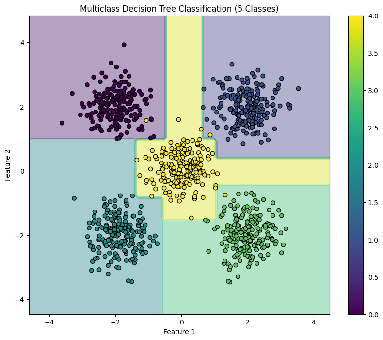
这种结构化方法演示了如何实现和评估多类分类任务的决策树,从而清楚地了解其功能和可视化决策边界的有效性。


